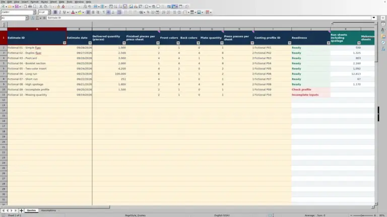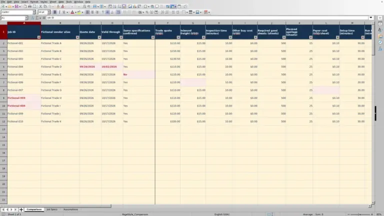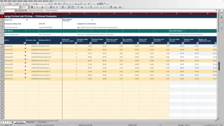
A change in run quantity can change which process costs less. The Print Shop Sheets digital versus offset break-even calculator compares two supplied cost curves so you can check the crossover and evaluate the quantities your customer is considering.
This editable Excel workbook uses a fixed setup cost and a run cost per delivered piece for each process. It is a cost comparison, not a full job estimate: you supply equivalent cost assumptions, then use the results to inform the process choice before completing your quote.
Where this workbook helps
- Compare alternative order quantities against the same digital and offset cost assumptions.
- See the mathematical crossover without manually solving the two cost equations.
- Read the cost difference and lower-cost process together for each valid quantity.
- Record the job description, assumption date and cost scope alongside the comparison.
What is in the file
How to get started
1. Describe the job and match the scope
On Inputs, replace the fictional Job description and Assumption date. Use Product and cost-scope notes to document the finished product and what each process cost includes. Check equivalent stock, finished dimensions, colors, finishing and included overhead.
2. Enter the two supplied cost curves
Enter each process's Setup cost (USD/job) and Run cost (USD/delivered piece). Costs must be numeric and nonnegative. The supplied run rates must already include applicable spoilage costs; the workbook does not calculate spoilage separately.
Set Same finished product and cost scope confirmed? to Yes only after reviewing both curves. Ready is an input-check result, not independent verification of the estimate.
3. Test the quantities under consideration
On Comparison, replace the fictional scenario labels and quantities in the cream input cells. Delivered quantity (pieces) must be a positive whole number, not gross sheets or impressions. The comparison provides 100 scenario rows using the same pair of cost curves.
4. Read the result before choosing a process
Check Mathematical crossover (delivered pieces), then review the total costs and Lower-cost process for your actual quantities. A positive Digital minus offset (USD) favors offset; a negative value favors digital. Open the file in Excel or LibreOffice to recalculate, and avoid overwriting the intentionally unprotected formulas.
Make the two supplied costs comparable first
The lower-cost result is useful only when both curves describe the same finished product and include equivalent costs. For example, comparing a digital cost that includes trimming with an offset cost that excludes it would not answer the process-choice question fairly.
Use Product and cost-scope notes on Inputs to make the basis visible. Identify the stock, finished dimensions, colors, finishing and included overhead. Then check that the supplied setup and run costs follow that basis for both processes. The workbook has aggregate cost inputs, not separate estimating lines for each component.
Keep the quantity basis consistent as well. Run cost is USD per delivered piece, with applicable spoilage already included in the supplied rate. Do not enter a cost per impression and treat it as a cost per finished piece, or add a second spoilage allowance to a rate that already includes one. Resolve any mismatch in your source estimate before confirming the scope.
Fictional example: finding the cost crossover
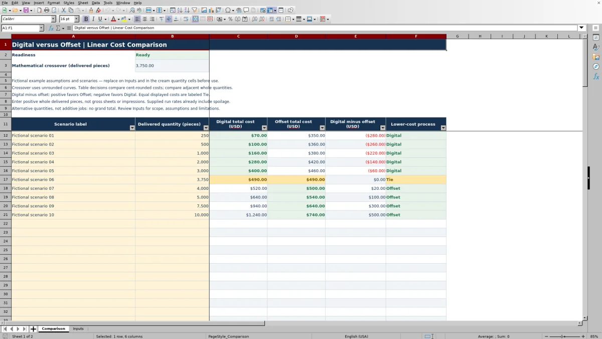
The workbook's fictional sample uses a digital setup cost of $40.00 per job and a run cost of $0.12 per delivered piece. Offset uses $340.00 per job and $0.04 per delivered piece. These are editable examples, not recommended shop rates.
For each process, total cost equals setup cost plus delivered quantity multiplied by run cost. At 3,000 delivered pieces, digital costs $40.00 + 3,000 × $0.12 = $400.00. Offset costs $340.00 + 3,000 × $0.04 = $460.00. Digital minus offset is −$60.00, so the row identifies Digital as the lower-cost process under these assumptions.
The crossover finds where the extra offset setup cost is balanced by its lower run cost: ($340.00 − $40.00) ÷ ($0.12 − $0.04) = 3,750 delivered pieces. Both curves cost $490.00 at that quantity. At 4,000 delivered pieces, digital costs $520.00 and offset costs $500.00, so the $20.00 positive difference favors Offset.
The next decision is to check the customer's likely order quantity against these results, then confirm that the cost assumptions still apply at that run length. The difference is a modeled cost difference, not profit or a promised saving.
Interpret fractional crossovers and no-crossover messages
The mathematical crossover uses the unrounded cost curves. It may fall between whole delivered quantities, but a fractional piece is not an order quantity. Enter the whole quantities immediately below and above that point in Comparison, along with the customer's requested quantity.
The row results compare costs rounded to cents. Close to the crossover, equal cent-rounded totals produce Tie even if the underlying unrounded costs differ slightly. Use those row results to understand the cost comparison at deliverable quantities rather than treating the mathematical crossover as an exact production instruction.
- All quantities tie means both setup costs and both run costs are equal.
- No crossover means the run costs are equal but the setup costs differ. The fixed cost gap remains at every quantity.
- No positive crossover means the curves meet at zero or a negative quantity, outside the positive delivered-quantity range.
When there is no positive crossover, use valid quantity rows to see which process costs less. Do not assume that offset must eventually become cheaper; the result depends on the costs you entered.
Troubleshooting blank results and misleading entries
Start with Readiness on Comparison if expected results are missing. Check inputs means at least one of the four setup or run costs is missing, nonnumeric or negative. Correct those entries on Inputs. A numeric zero is allowed, but a blank cost is not a substitute for zero.
Confirm scope means the confirmation field is not set to Yes. Review the scope rather than changing the answer merely to display results. Once the costs pass the checks and scope is confirmed, Readiness shows Ready.
If Readiness is Ready but an individual row remains blank, check its Delivered quantity (pieces). Text, zero, negative values and fractional quantities do not produce row results. A blank output is not a zero-cost job; correct the input before interpreting it.
If totals appear unchanged after editing, recalculate in Excel or LibreOffice. If a calculated cell was accidentally overwritten, return to an intact copy of the workbook and re-enter your inputs. The formulas are intentionally unprotected, so keeping an untouched original is a useful precaution.
Know when the linear model no longer fits the run
This comparison assumes a fixed setup cost plus a constant run cost per delivered piece. Increasing quantity changes only the quantity multiplied by that rate. It does not add another setup, apply a supplier price tier or change the rate when equipment capacity is reached.
One straight-line cost curve may not fit every run length. If your source estimate changes its rate or setup basis at a quantity threshold, use assumptions appropriate to the range you are evaluating. Keep separate copies for distinct cost regimes, and interpret each crossover only within the range where its assumptions apply.
The workbook does not calculate paper consumption, imposition, capacity, selling price, tax or schedule. A lower modeled cost therefore does not establish that the process can meet the stock requirement or due date. Check those constraints separately before making the production commitment.
Compare this workbook with a blank spreadsheet
A blank spreadsheet can support the same arithmetic if you build and check it. The choice depends on whether you need this defined two-process comparison or a different estimating structure.
| Method | Cost model | Input and scope checks | Quantity review | Ongoing work |
|---|---|---|---|---|
| Print Shop Sheets workbook | Fixed setup plus a constant run cost for each of two processes; no full estimating breakdown. | Checks four costs and requires a Yes scope confirmation; you still assess equivalence. | Provides a crossover and 100 rows with total costs, differences and lower-cost labels. | Replace assumptions and quantities, preserve formulas and keep dated copies as needed. |
| Blank spreadsheet built by your shop | You define the structure, including any cost tiers or additional components you need. | You must create any checks and document how scope is confirmed. | You must build and verify the crossover and quantity comparisons you want. | You maintain the formulas, layout and assumptions you create. |
Use this workbook when you already have two comparable linear cost curves and need a focused quantity comparison. Consider a custom spreadsheet when the decision requires tiered costs or a different model, provided your shop can build and maintain those calculations. Neither approach removes the need to check the source costs.
Keep the comparison clear at the estimating handoff
The scenario rows are alternative quantities for one shared set of assumptions, not additive jobs. There is no grand total. Changing a setup or run cost on Inputs affects all valid comparison rows, so different scenario labels do not give each row its own rates.
Before revising an assumption, keep a dated copy if you need to preserve the earlier comparison. Update Assumption date and the scope notes in the working copy so the next person can identify the basis used. Do not treat an overwritten input as retained history.
At handoff, identify the selected delivered quantity, the modeled cost difference and any unresolved production constraint. Carry the result into your normal quoting process; this workbook applies no markup or margin and does not turn the selected process cost into a customer selling price.
Frequently asked questions
Does break-even mean the job becomes profitable at that quantity?
No. Here, break-even means the digital and offset cost curves are equal. The workbook has no selling-price, markup or margin calculation, so it does not identify a profit threshold.
Can I use zero for a setup cost or run cost?
Yes. Numeric zero is a valid cost input. Use it only when it reflects the supplied cost basis, not when the cost is unknown. Missing, nonnumeric or negative cost inputs cause Check inputs.
Does the workbook include a graph of the cost curves?
No. It presents the mathematical crossover and quantity-by-quantity results in cells. There is no built-in chart.
Can I open the workbook in LibreOffice?
The workbook instructions specify Excel or LibreOffice for recalculation. Open it in one of those applications and check the recalculated results after entering your assumptions; a static preview is not a substitute for recalculation.
Are the supplied rates and product details real shop data?
No. The included assumptions and scenarios are fictional. Replace the costs, job description, assumption date, scope notes and scenario quantities before using the comparison for a live job. The USD inputs are editable assumptions, not live supplier prices.
Editorial coverage

Clara WinslowPrint estimating editor

Miles FenwickPrint workflow editor